Machine Learning

Intro & Linear regression with one variable

supervised learning & unsupervised learning

supervised learning: learn from labeled data. input $\rightarrow$ output
- regression
- classification
unsupervised learning: only unlabeled data
- cluster
- dimensionality reduction
- anomaly detection

linear regression

$y=wx+b$

training set: data used to train the model
cost function:

$J(w,b)=\frac{1}{2m}\sum_{i=1}^{m}(\hat{y}^{(i)}-{y}^{(i)})^2$
- goal: minimize $J$
- it’s a bowl shape surface

gradient descent

how to move downhill

algorithm

$w \leftarrow{w}-\alpha\frac{\partial}{\partial{w}}J(w,b)$

$b\leftarrow{b}-\alpha\frac{\partial}{\partial{b}}J(w,b)$

$\frac{\partial}{\partial{w}}J(w,b)=\frac{1}{m}\sum_{i=1}^{m}(\hat{y}^{(i)}-{y}^{(i)})x^{(i)}$

$\frac{\partial}{\partial{b}}J(w,b)=\frac{1}{m}\sum_{i=1}^{m}(\hat{y}^{(i)}-{y}^{(i)})$

where $\alpha$ is the learning rate, which is between 0 and 1. It’s the degree of how large the step downhill we take. if $\alpha$ is too small, gradient descent will be slow. if $\alpha$ is too large, you will get overshoot.

repeat until convergence

batch gradient descent: each step uses all training data

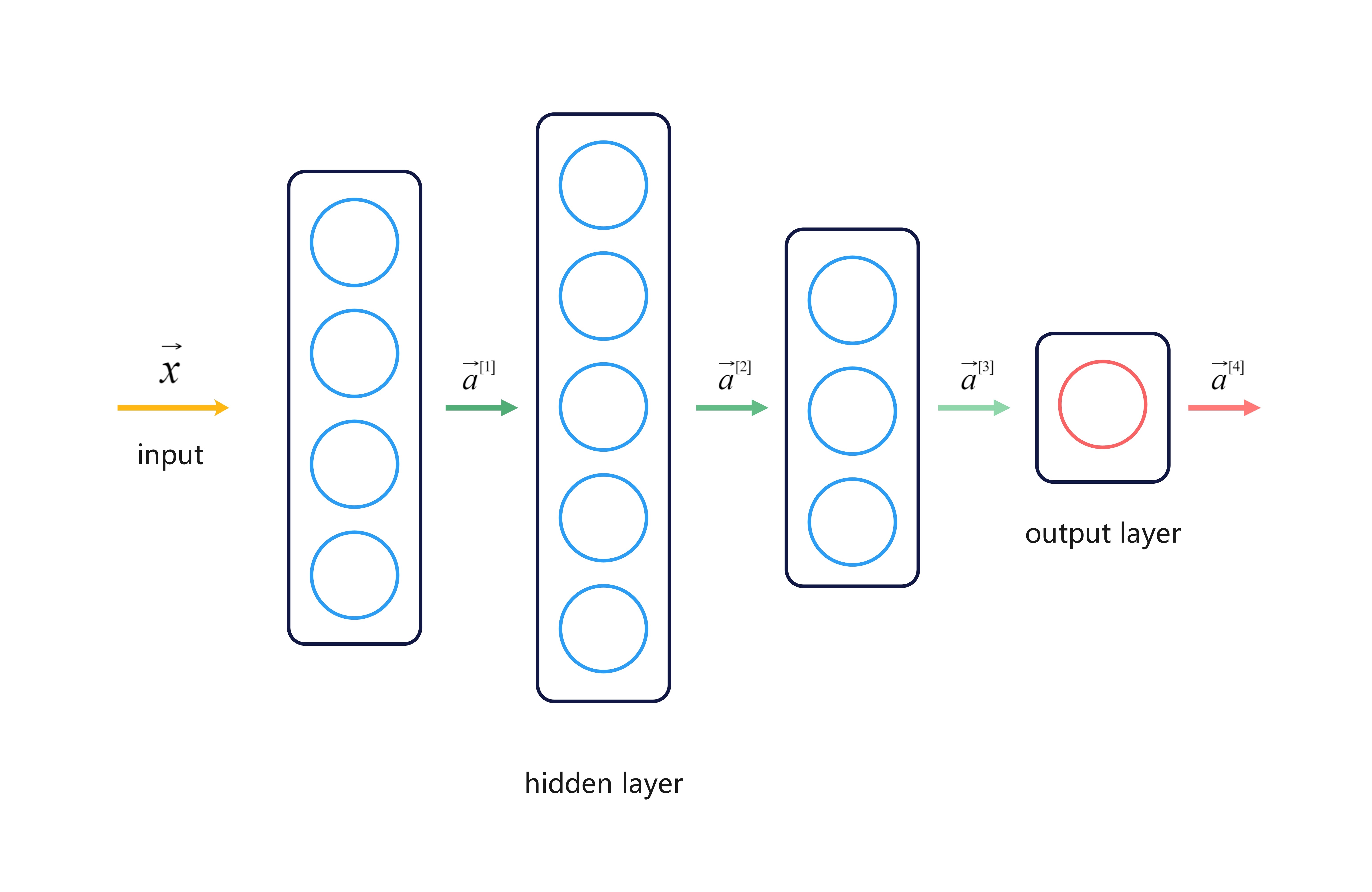
Linear regression with multiple variables

multiple features

use vectors

$f_{\overrightarrow{w},b}(\ \overrightarrow{x}\ )=\overrightarrow{w}\cdot\overrightarrow{x}+b$

vectorization (with numpy)
1
f=np.dot(w,x)+b
- compared to loops, it’s a more efficient way
normal equation
- only for linear equation to find w,b without iterations

feature scaling

make gradient descent faster

Z-score normalization
$x_1=\frac{x_1-\mu_1}{\sigma_1}$

check convergence

if $J(\overrightarrow{w},b)$ decreases by $\leqslant\epsilon$ , we declare convergence

feature engineering

design features

polynomial regression

with scikit-learn

Classification

binary classification: true(1) or false(0)

logistic regression

sigmoid function:

$g(z)=\frac{1}{1+e^{-z}}$

logistic regression
$f_{\overrightarrow{w},b}(\ \overrightarrow{x}\ )=\frac{1}{1+e^{-(\overrightarrow{w}\ \cdot\ \overrightarrow{x}+b)}}$

decision boundary

the line that is neutral (threshold is 0.5) about y=0 or y=1

$z=\overrightarrow{w}\cdot\overrightarrow{x}+b=0$

cost function

if we use the squared error cost which is the same as linear regression, we will get a non-convex curve.

loss function

measures how well we are doing on one training examples
- loss function for squared error cost
  
  $L(f_{\overrightarrow{w},b}(\ \overrightarrow{x}\ ^{(i)}),y^{(i)})=\frac{1}{2}(f_{\overrightarrow{w},b}(\ \overrightarrow{x}\ ^{(i)})-y^{(i)})^2$
- logistic loss function
  
  $L(f_{\overrightarrow{w},b}(\ \overrightarrow{x}\ ^{(i)}),y^{(i)})=\left\{\begin{array}{rcl}-log(f_{\overrightarrow{w},b}(\ \overrightarrow{x}\ ^{(i)}))&if\ \ y^{(i)}=1\\-log(1-f_{\overrightarrow{w},b}(\ \overrightarrow{x}\ ^{(i)}))&if\ \ y^{(i)}=0 \end{array}\right.$
  - $y^{(i)}=1$
    
    $loss\rightarrow 0\ \ as\ \ f_{\overrightarrow{w},b}(\ \overrightarrow{x}\ ^{(i)})\rightarrow1$
  - $y^{(i)}=0$
    
    $loss\rightarrow 0\ \ as\ \ f_{\overrightarrow{w},b}(\ \overrightarrow{x}\ ^{(i)})\rightarrow0$
cost function

$J(\overrightarrow{w},b)=\frac{1}{m}\sum_{i=1}^{m}L(f_{\overrightarrow{w},b}(\ \overrightarrow{x}\ ^{(i)}),y^{(i)})$
simplified loss function

$L(f_{\overrightarrow{w},b}(\ \overrightarrow{x}\ ^{(i)}),y^{(i)})=-y^{(i)}log(f_{\overrightarrow{w},b}(\ \overrightarrow{x}\ ^{(i)}))-(1-y^{(i)})log(1-f_{\overrightarrow{w},b}(\ \overrightarrow{x}\ ^{(i)}))$
simplified cost function

$J(\overrightarrow{w},b)=-\frac{1}{m}\sum_{i=1}^m[y^{(i)}log(f_{\overrightarrow{w},b}(\ \overrightarrow{x}\ ^{(i)}))+(1-y^{(i)})log(1-f_{\overrightarrow{w},b}(\ \overrightarrow{x}\ ^{(i)}))]$

gradient descent

$\frac{\partial}{\partial{w_j}}J(\overrightarrow{w},b)=\frac{1}{m}\sum_{i=1}^{m}(f_{\overrightarrow{w},b}(\ \overrightarrow{x}\ ^{(i)})-{y}^{(i)})x_j^{(i)}\ \ (*)\\ \frac{\partial}{\partial{b}}J(\overrightarrow{w},b)=\frac{1}{m}\sum_{i=1}^{m}(f_{\overrightarrow{w},b}(\ \overrightarrow{x}\ ^{(i)})-{y}^{(i)})$

how to get $(*)$
$\begin{align} \frac{\partial}{\partial{w_j}}J(\overrightarrow{w},b)&=-\frac{1}{m}\sum_{i=1}^m(\frac{y^{(i)}}{f}-\frac{1-y^{(i)}}{1-f})\frac{\partial{f}}{\partial{w_j}}\nonumber\\ &=-\frac{1}{m}\sum_{i=1}^{m}\frac{y^{(i)}-f}{f(1-f)}\cdot\frac{\partial{f}}{\partial{w_j}}\nonumber\\ &=-\frac{1}{m}\sum_{i=1}^{m}\frac{y^{(i)}-f}{f(1-f)}f(1-f)x_j^{(i)}\nonumber\\ &=\frac{1}{m}\sum_{i=1}^{m}(f-{y}^{(i)})x_j^{(i)}\nonumber \end{align}$
where $f=\frac{1}{1+e^{-(\overrightarrow{w}\ \cdot\ \overrightarrow{x}\ ^{(i)}+b)}}$

overfitting

high variance

fits the training set extremely well

how to address it
- collect more training examples
- select features to include/ exclude
- regularization: reduce the size of parameter $w_j$
regularization

$\min_{\overrightarrow{w},b}J(\overrightarrow{w},b)=\min_{\overrightarrow{w},b}[\frac{1}{2m}\sum_{i=1}^{m}L(f_{\overrightarrow{w},b}(\ \overrightarrow{x}\ ^{(i)})-y^{(i)})^2+\frac{\lambda}{2m}\sum_{j=1}^{n}w_j^2]$
- gradient descent
  $w_j\leftarrow{w_j}(1-\alpha\frac{\lambda}{m})-\alpha\frac{1}{m}\sum_{i=1}^{m}(f_{\overrightarrow{w},b}(\ \overrightarrow{x}\ ^{(i)})-{y}^{(i)})x_j^{(i)}\\ b\leftarrow{b}-\alpha\frac{1}{m}\sum_{i=1}^{m}(f_{\overrightarrow{w},b}(\ \overrightarrow{x}\ ^{(i)})-{y}^{(i)})$

Neural network

dense: every neuron gets its inputs all the activations from the previous layer.

$\overrightarrow{x}=\overrightarrow{a}\ _j^{[0]}\\ a_j^{[l]}=g(\overrightarrow{w}\ _j^{[l]}\cdot\overrightarrow{a}\ ^{[l-1]}+b_j^{[l]})$

where $a_j^{[l]}$ is the activation value of layer $l$ , unit $j$ . $g$ is sigmoid function (a activation function).

forward propagation

def dense(a_in,W,b,g):
	units=W.shape[1] 
	a_out=np.zeros(units)
	for j in range(units):
        w=W[:,j]
        z=np.dot(w,a_in)+b[j]
        a_out[j]=g(z)
    return a_out


#simplication
def dense(AT,W,b,g):
    z=np.matmul(AT,W)+b
    a_out=g(z)
    return a_out


def sequential(x):
    a1=dense(x,W1,b1)
    a2=dense(a1,W2,b2)
    a3=dense(a2,W3,b3)
    a4=dense(a3,W4,b4)
    f_x=a4
    return f_x

matrix multiplication

$Z=A^TW$

1
2
3

Z=np.matmul(AT,W)
#or
Z=AT@W

sample code

from tensorflow.python.keras.layers import Dense
from tensorflow.python.keras import Sequential
from tensorflow.python.keras.losses import BinaryCrossentropy

model=Sequential([
    Dense(units=25,activation='sigmoid'),
    Dense(units=15,activation='sigmoid'),
    Dense(units=1,activation='sigmoid')
])

model.compile(loss=BinaryCrossentropy)
model.fit(X,Y,epochs=100)

activation function

linear (also means no activation function)
- output: +/-
sigmoid
- output: 0/1
ReLU

$g(z)=max(0,z)$
- output: 0/+
- most common choice
  - faster
  - only one side flat. flat is slow for gradient descent.

activation function issue

why we use activation function?

use linear function for all hidden layers and output layer $\Longleftrightarrow$ linear regression
use linear function for all hidden layers but sigmoid function for output layer $\Longleftrightarrow$ logistic regression

adam algorithm

Adaptive Moment estimation (not just one $\alpha$ )

1	model.compile(optimizer=Adam(learning_rate=1e-3),loss=...)

convolutional neural network

convolutional layer

Each neuron only looks at part of the previous layer’s inputs.

why
- faster
- less training data

Muticlass Classification

softmax

$z_j=\overrightarrow{w}_j\cdot\overrightarrow{x}+b_j\ \ \ \ \ j=1,...,N\\ a_j=\frac{e^{z_j}}{\sum_{k=1}^Ne^{z_k}}=P(y=j|\ \overrightarrow{x}\ )$

loss function

$loss(a_1,...,a_N,y)=\left\{\begin{array}{rcl}-log(a_1)&if\ \ y=1\\ -log(a_2)&if\ \ y=2\\ \vdots \\-log(a_N)&if\ \ y=N \end{array}\right.$

sample code

from tensorflow.python.keras.layers import Dense
from tensorflow.python.keras import Sequential
from tensorflow.python.keras.losses import SparseCategoricalCrossentropy

model=Sequential([
    Dense(units=25,activation='relu'),
    Dense(units=15,activation='relu'),
    Dense(units=1,activation='linear')
])
#More numercially accurate implementation of softmax
model.compile(loss=SparseCategoricalCrossentropy(from_logits=True))
model.fit(X,Y,epochs=100)

Evaluating a model

training set --60%
cross validation set --20%
- $J_{cv}(\overrightarrow{w},b)$ is used to select a model, pick a set of parameters
test set --20%
- $J_{test}(\overrightarrow{w},b)$ is better estimate of how well the model will generalize to new data

The error does not contain regularization term

$J_{test}(\overrightarrow{w},b)$ is better estimate of how well the model will generalize to new data

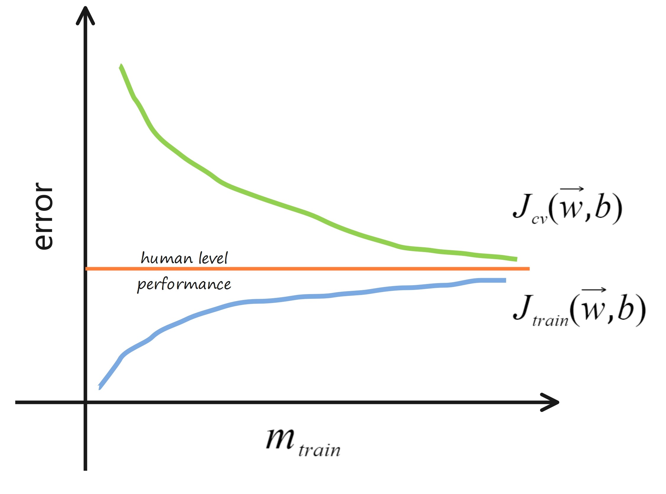
bias & variance

high bias – underfit $\leftarrow$ $J_{train}(\overrightarrow{w},b)$ is high, $J_{cv}(\overrightarrow{w},b)$ is high
just right $\leftarrow$ $J_{train}(\overrightarrow{w},b)$ is low, $J_{cv}(\overrightarrow{w},b)$ is low
high variance – overfit $\leftarrow$ $J_{train}(\overrightarrow{w},b)$ is low, $J_{cv}(\overrightarrow{w},b)$ is high

regularization issue

large $\lambda$ $\Rightarrow$ high bias
small $\lambda$ $\Rightarrow$ high variance

learning curve

Decision trees

choose feature to be split on – maximize purity
when to stop?
- a node is 100% one class
- exceeding a maximum depth
- improvement in purity score is below a threshold
- number of examples in a node is below a threshold